c++ - paso - ¿Cómo detectar un árbol de navidad?
ideas de como decorar el arbol de navidad elegante (10)
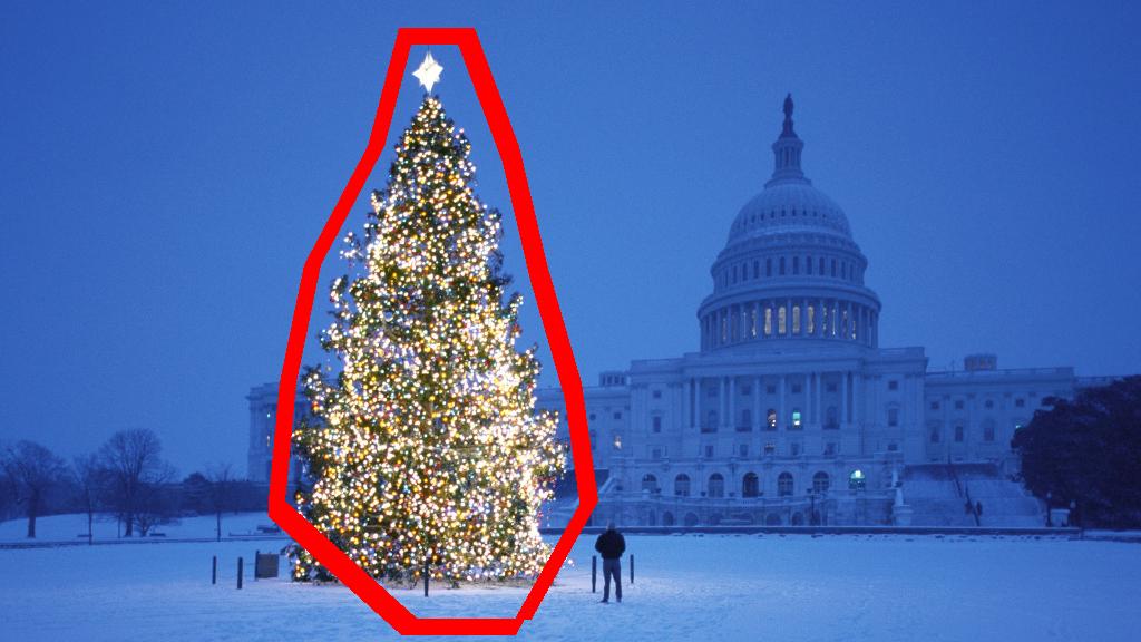
¿Qué técnicas de procesamiento de imágenes podrían usarse para implementar una aplicación que detecte los árboles de navidad que se muestran en las siguientes imágenes?
Estoy buscando soluciones que funcionen en todas estas imágenes. Por lo tanto, los enfoques que requieren entrenamiento de clasificadores en cascada o la combinación de plantillas no son muy interesantes.
Estoy buscando algo que se pueda escribir en cualquier lenguaje de programación, siempre y cuando use solo tecnologías de código abierto . La solución se debe probar con las imágenes que se comparten en esta pregunta. Hay 6 imágenes de entrada y la respuesta debe mostrar los resultados del procesamiento de cada una de ellas. Finalmente, para cada imagen de salida debe haber líneas rojas dibujadas para rodear el árbol detectado.
¿Cómo harías para detectar programáticamente los árboles en estas imágenes?
Aquí está mi solución simple y tonta. Se basa en la suposición de que el árbol será la cosa más brillante y grande de la imagen.
//g++ -Wall -pedantic -ansi -O2 -pipe -s -o christmas_tree christmas_tree.cpp `pkg-config --cflags --libs opencv`
#include <opencv2/imgproc/imgproc.hpp>
#include <opencv2/highgui/highgui.hpp>
#include <iostream>

using namespace cv;
using namespace std;

int main(int argc,char *argv[])
{
    Mat original,tmp,tmp1;
    vector <vector<Point> > contours;
    Moments m;
    Rect boundrect;
    Point2f center;
    double radius, max_area=0,tmp_area=0;
    unsigned int j, k;
    int i;

    for(i = 1; i < argc; ++i)
    {
        original = imread(argv[i]);
        if(original.empty())
        {
            cerr << "Error"<<endl;
            return -1;
        }

        GaussianBlur(original, tmp, Size(3, 3), 0, 0, BORDER_DEFAULT);
        erode(tmp, tmp, Mat(), Point(-1, -1), 10);
        cvtColor(tmp, tmp, CV_BGR2HSV);
        inRange(tmp, Scalar(0, 0, 0), Scalar(180, 255, 200), tmp);

        dilate(original, tmp1, Mat(), Point(-1, -1), 15);
        cvtColor(tmp1, tmp1, CV_BGR2HLS);
        inRange(tmp1, Scalar(0, 185, 0), Scalar(180, 255, 255), tmp1);
        dilate(tmp1, tmp1, Mat(), Point(-1, -1), 10);

        bitwise_and(tmp, tmp1, tmp1);

        findContours(tmp1, contours, CV_RETR_EXTERNAL, CV_CHAIN_APPROX_SIMPLE);
        max_area = 0;
        j = 0;
        for(k = 0; k < contours.size(); k++)
        {
            tmp_area = contourArea(contours[k]);
            if(tmp_area > max_area)
            {
                max_area = tmp_area;
                j = k;
            }
        }
        tmp1 = Mat::zeros(original.size(),CV_8U);
        approxPolyDP(contours[j], contours[j], 30, true);
        drawContours(tmp1, contours, j, Scalar(255,255,255), CV_FILLED);

        m = moments(contours[j]);
        boundrect = boundingRect(contours[j]);
        center = Point2f(m.m10/m.m00, m.m01/m.m00);
        radius = (center.y - (boundrect.tl().y))/4.0*3.0;
        Rect heightrect(center.x-original.cols/5, boundrect.tl().y, original.cols/5*2, boundrect.size().height);

        tmp = Mat::zeros(original.size(), CV_8U);
        rectangle(tmp, heightrect, Scalar(255, 255, 255), -1);
        circle(tmp, center, radius, Scalar(255, 255, 255), -1);

        bitwise_and(tmp, tmp1, tmp1);

        findContours(tmp1, contours, CV_RETR_EXTERNAL, CV_CHAIN_APPROX_SIMPLE);
        max_area = 0;
        j = 0;
        for(k = 0; k < contours.size(); k++)
        {
            tmp_area = contourArea(contours[k]);
            if(tmp_area > max_area)
            {
                max_area = tmp_area;
                j = k;
            }
        }

        approxPolyDP(contours[j], contours[j], 30, true);
        convexHull(contours[j], contours[j]);

        drawContours(original, contours, j, Scalar(0, 0, 255), 3);

        namedWindow(argv[i], CV_WINDOW_NORMAL|CV_WINDOW_KEEPRATIO|CV_GUI_EXPANDED);
        imshow(argv[i], original);

        waitKey(0);
        destroyWindow(argv[i]);
    }

    return 0;
}
El primer paso es detectar los píxeles más brillantes de la imagen, pero tenemos que hacer una distinción entre el árbol en sí y la nieve que refleja su luz. Aquí intentamos excluir la aplicación de nieve con un filtro realmente simple en los códigos de color:
GaussianBlur(original, tmp, Size(3, 3), 0, 0, BORDER_DEFAULT);
erode(tmp, tmp, Mat(), Point(-1, -1), 10);
cvtColor(tmp, tmp, CV_BGR2HSV);
inRange(tmp, Scalar(0, 0, 0), Scalar(180, 255, 200), tmp);
Luego encontramos cada píxel "brillante":
dilate(original, tmp1, Mat(), Point(-1, -1), 15);
cvtColor(tmp1, tmp1, CV_BGR2HLS);
inRange(tmp1, Scalar(0, 185, 0), Scalar(180, 255, 255), tmp1);
dilate(tmp1, tmp1, Mat(), Point(-1, -1), 10);
Finalmente unimos los dos resultados:
bitwise_and(tmp, tmp1, tmp1);
Ahora buscamos el objeto brillante más grande:
findContours(tmp1, contours, CV_RETR_EXTERNAL, CV_CHAIN_APPROX_SIMPLE);
max_area = 0;
j = 0;
for(k = 0; k < contours.size(); k++)
{
    tmp_area = contourArea(contours[k]);
    if(tmp_area > max_area)
    {
        max_area = tmp_area;
        j = k;
    }
}
tmp1 = Mat::zeros(original.size(),CV_8U);
approxPolyDP(contours[j], contours[j], 30, true);
drawContours(tmp1, contours, j, Scalar(255,255,255), CV_FILLED);
Ya casi hemos terminado, pero todavía hay algunas imperfecciones debido a la nieve. Para cortarlos, construiremos una máscara utilizando un círculo y un rectángulo para aproximar la forma de un árbol para eliminar piezas no deseadas:
m = moments(contours[j]);
boundrect = boundingRect(contours[j]);
center = Point2f(m.m10/m.m00, m.m01/m.m00);
radius = (center.y - (boundrect.tl().y))/4.0*3.0;
Rect heightrect(center.x-original.cols/5, boundrect.tl().y, original.cols/5*2, boundrect.size().height);

tmp = Mat::zeros(original.size(), CV_8U);
rectangle(tmp, heightrect, Scalar(255, 255, 255), -1);
circle(tmp, center, radius, Scalar(255, 255, 255), -1);

bitwise_and(tmp, tmp1, tmp1);
El último paso es encontrar el contorno de nuestro árbol y dibujarlo en la imagen original.
findContours(tmp1, contours, CV_RETR_EXTERNAL, CV_CHAIN_APPROX_SIMPLE);
max_area = 0;
j = 0;
for(k = 0; k < contours.size(); k++)
{
    tmp_area = contourArea(contours[k]);
    if(tmp_area > max_area)
    {
        max_area = tmp_area;
        j = k;
    }
}

approxPolyDP(contours[j], contours[j], 30, true);
convexHull(contours[j], contours[j]);

drawContours(original, contours, j, Scalar(0, 0, 255), 3);
Lo siento, pero en este momento tengo una mala conexión, por lo que no puedo subir fotos. Intentaré hacerlo más tarde.
Feliz Navidad.
EDITAR:
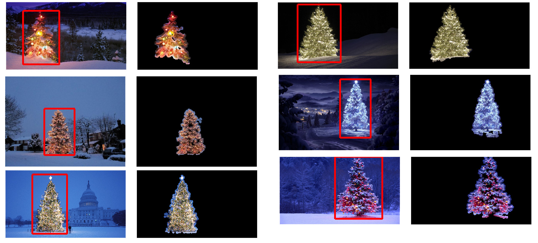
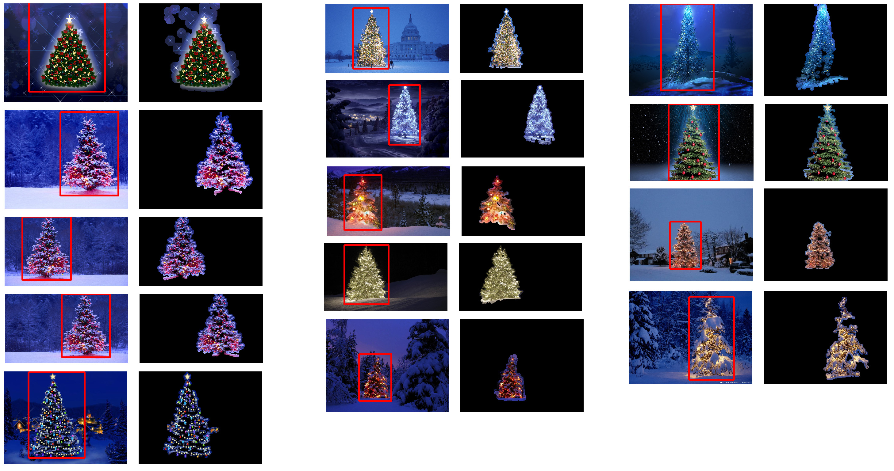
Aquí algunas fotos de la salida final:
Escribí el código en Matlab R2007a. Usé k-medias para extraer aproximadamente el árbol de navidad. Mostraré mi resultado intermedio solo con una imagen y los resultados finales con las seis.
Primero, asigné el espacio RGB al espacio Lab, lo que podría mejorar el contraste del rojo en su canal b:
colorTransform = makecform(''srgb2lab'');
I = applycform(I, colorTransform);
L = double(I(:,:,1));
a = double(I(:,:,2));
b = double(I(:,:,3));
Además de la función en el espacio de color, también usé la función de textura que es relevante para el vecindario en lugar de cada píxel. Aquí combiné linealmente la intensidad de los 3 canales originales (R, G, B). La razón por la que formateé de esta manera es porque los árboles de navidad en la imagen tienen luces rojas, y algunas veces también iluminación verde / a veces azul.
R=double(Irgb(:,:,1));
G=double(Irgb(:,:,2));
B=double(Irgb(:,:,3));
I0 = (3*R + max(G,B)-min(G,B))/2;
Apliqué un patrón binario local 3X3 en I0 , usé el píxel central como umbral y obtuve el contraste calculando la diferencia entre el valor de la intensidad de píxel media por encima del umbral y el valor de la media por debajo.
I0_copy = zeros(size(I0));
for i = 2 : size(I0,1) - 1
    for j = 2 : size(I0,2) - 1
        tmp = I0(i-1:i+1,j-1:j+1) >= I0(i,j);
        I0_copy(i,j) = mean(mean(tmp.*I0(i-1:i+1,j-1:j+1))) - ...
            mean(mean(~tmp.*I0(i-1:i+1,j-1:j+1))); % Contrast
    end
end
Como tengo 4 funciones en total, elegiría K = 5 en mi método de agrupación. El código para k-means se muestra a continuación (es del curso de aprendizaje automático del Dr. Andrew Ng. Tomé el curso anteriormente y escribí el código yo mismo en su asignación de programación).
[centroids, idx] = runkMeans(X, initial_centroids, max_iters);
mask=reshape(idx,img_size(1),img_size(2));

%%%%%%%%%%%%%%%%%%%%%%%%%%%%%%%%%%%%%%%%%%%%%%%%%%%%
function [centroids, idx] = runkMeans(X, initial_centroids, ...
                                  max_iters, plot_progress)
   [m n] = size(X);
   K = size(initial_centroids, 1);
   centroids = initial_centroids;
   previous_centroids = centroids;
   idx = zeros(m, 1);

   for i=1:max_iters
      % For each example in X, assign it to the closest centroid
      idx = findClosestCentroids(X, centroids);

      % Given the memberships, compute new centroids
      centroids = computeCentroids(X, idx, K);

   end
%%%%%%%%%%%%%%%%%%%%%%%%%%%%%%%%%%%%%%%%%%%%%%%%%%%%%%%
function idx = findClosestCentroids(X, centroids)
   K = size(centroids, 1);
   idx = zeros(size(X,1), 1);
   for xi = 1:size(X,1)
      x = X(xi, :);
      % Find closest centroid for x.
      best = Inf;
      for mui = 1:K
        mu = centroids(mui, :);
        d = dot(x - mu, x - mu);
        if d < best
           best = d;
           idx(xi) = mui;
        end
      end
   end
%%%%%%%%%%%%%%%%%%%%%%%%%%%%%%%%%%%
function centroids = computeCentroids(X, idx, K)
   [m n] = size(X);
   centroids = zeros(K, n);
   for mui = 1:K
      centroids(mui, :) = sum(X(idx == mui, :)) / sum(idx == mui);
   end
Como el programa se ejecuta muy lento en mi computadora, acabo de ejecutar 3 iteraciones. Normalmente, el criterio de detención es (i) el tiempo de iteración de al menos 10, o (ii) ya no hay cambios en los centroides. Para mi prueba, aumentar la iteración puede diferenciar el fondo (cielo y árbol, cielo y edificio, ...) con mayor precisión, pero no mostró cambios drásticos en la extracción del árbol de Navidad. También tenga en cuenta que k-means no es inmune a la inicialización aleatoria de centroide, por lo que se recomienda ejecutar el programa varias veces para hacer una comparación.
Después de las medias k, se eligió la región marcada con la intensidad máxima de I0 . Y el trazado de límites se utilizó para extraer los límites. Para mí, el último árbol de Navidad es el más difícil de extraer ya que el contraste en esa imagen no es lo suficientemente alto como lo son en los primeros cinco. Otro problema en mi método es que bwboundaries función bwboundaries en Matlab para trazar el límite, pero a veces también se incluyen los límites internos, como se puede observar en los resultados 3, 5 y 6 The dark side within the christmas trees are not only failed to be clustered with the illuminated side, but they also lead to so many tiny inner boundaries tracing ( imfill doesn''t improve very much). In all my algorithm still has a lot improvement space.
Some publication s indicates that mean-shift may be more robust than k-means, and many graph-cut based algorithms are also very competitive on complicated boundaries segmentation. I wrote a mean-shift algorithm myself, it seems to better extract the regions without enough light. But mean-shift is a little bit over-segmented, and some strategy of merging is needed. It ran even much slower than k-means in my computer, I am afraid I have to give it up. I eagerly look forward to see others would submit excellent results here with those modern algorithms mentioned above.
Yet I always believe the feature selection is the key component in image segmentation. With a proper feature selection that can maximize the margin between object and background, many segmentation algorithms will definitely work. Different algorithms may improve the result from 1 to 10, but the feature selection may improve it from 0 to 1.
Feliz Navidad !
NOTA DE EDICIÓN: edité esta publicación para (i) procesar cada imagen de árbol individualmente, como se solicita en los requisitos, (ii) para considerar tanto el brillo como la forma del objeto para mejorar la calidad del resultado.
A continuación se presenta un enfoque que toma en consideración el brillo y la forma del objeto. En otras palabras, busca objetos con forma de triángulo y con un brillo significativo. Se implementó en Java, utilizando el marco de procesamiento de imágenes Marvin .
El primer paso es el umbral de color. El objetivo aquí es enfocar el análisis en objetos con brillo significativo.
imágenes de salida:
http://marvinproject.sourceforge.net/other/trees/tree_1threshold.png http://marvinproject.sourceforge.net/other/trees/tree_2threshold.png http://marvinproject.sourceforge.net/other/trees/tree_3threshold.png
http://marvinproject.sourceforge.net/other/trees/tree_4threshold.png http://marvinproject.sourceforge.net/other/trees/tree_5threshold.png http://marvinproject.sourceforge.net/other/trees/tree_6threshold.png
código fuente:
public class ChristmasTree {

private MarvinImagePlugin fill = MarvinPluginLoader.loadImagePlugin("org.marvinproject.image.fill.boundaryFill");
private MarvinImagePlugin threshold = MarvinPluginLoader.loadImagePlugin("org.marvinproject.image.color.thresholding");
private MarvinImagePlugin invert = MarvinPluginLoader.loadImagePlugin("org.marvinproject.image.color.invert");
private MarvinImagePlugin dilation = MarvinPluginLoader.loadImagePlugin("org.marvinproject.image.morphological.dilation");

public ChristmasTree(){
    MarvinImage tree;

    // Iterate each image
    for(int i=1; i<=6; i++){
        tree = MarvinImageIO.loadImage("./res/trees/tree"+i+".png");

        // 1. Threshold
        threshold.setAttribute("threshold", 200);
        threshold.process(tree.clone(), tree);
    }
}
public static void main(String[] args) {
    new ChristmasTree();
}
}
En el segundo paso, los puntos más brillantes de la imagen se dilatan para formar formas. El resultado de este proceso es la forma probable de los objetos con brillo significativo. Aplicando la segmentación de relleno de inundación, se detectan formas desconectadas.
imágenes de salida:
http://marvinproject.sourceforge.net/other/trees/tree_1_fill.png http://marvinproject.sourceforge.net/other/trees/tree_2_fill.png http://marvinproject.sourceforge.net/other/trees/tree_3_fill.png
http://marvinproject.sourceforge.net/other/trees/tree_4_fill.png http://marvinproject.sourceforge.net/other/trees/tree_5_fill.png http://marvinproject.sourceforge.net/other/trees/tree_6_fill.png
código fuente:
public class ChristmasTree {

private MarvinImagePlugin fill = MarvinPluginLoader.loadImagePlugin("org.marvinproject.image.fill.boundaryFill");
private MarvinImagePlugin threshold = MarvinPluginLoader.loadImagePlugin("org.marvinproject.image.color.thresholding");
private MarvinImagePlugin invert = MarvinPluginLoader.loadImagePlugin("org.marvinproject.image.color.invert");
private MarvinImagePlugin dilation = MarvinPluginLoader.loadImagePlugin("org.marvinproject.image.morphological.dilation");

public ChristmasTree(){
    MarvinImage tree;

    // Iterate each image
    for(int i=1; i<=6; i++){
        tree = MarvinImageIO.loadImage("./res/trees/tree"+i+".png");

        // 1. Threshold
        threshold.setAttribute("threshold", 200);
        threshold.process(tree.clone(), tree);

        // 2. Dilate
        invert.process(tree.clone(), tree);
        tree = MarvinColorModelConverter.rgbToBinary(tree, 127);
        MarvinImageIO.saveImage(tree, "./res/trees/new/tree_"+i+"threshold.png");
        dilation.setAttribute("matrix", MarvinMath.getTrueMatrix(50, 50));
        dilation.process(tree.clone(), tree);
        MarvinImageIO.saveImage(tree, "./res/trees/new/tree_"+1+"_dilation.png");
        tree = MarvinColorModelConverter.binaryToRgb(tree);

        // 3. Segment shapes
        MarvinImage trees2 = tree.clone();
        fill(tree, trees2);
        MarvinImageIO.saveImage(trees2, "./res/trees/new/tree_"+i+"_fill.png");
}

private void fill(MarvinImage imageIn, MarvinImage imageOut){
    boolean found;
    int color= 0xFFFF0000;

    while(true){
        found=false;

        Outerloop:
        for(int y=0; y<imageIn.getHeight(); y++){
            for(int x=0; x<imageIn.getWidth(); x++){
                if(imageOut.getIntComponent0(x, y) == 0){
                    fill.setAttribute("x", x);
                    fill.setAttribute("y", y);
                    fill.setAttribute("color", color);
                    fill.setAttribute("threshold", 120);
                    fill.process(imageIn, imageOut);
                    color = newColor(color);

                    found = true;
                    break Outerloop;
                }
            }
        }

        if(!found){
            break;
        }
    }

}

private int newColor(int color){
    int red = (color & 0x00FF0000) >> 16;
    int green = (color & 0x0000FF00) >> 8;
    int blue = (color & 0x000000FF);

    if(red <= green && red <= blue){
        red+=5;
    }
    else if(green <= red && green <= blue){
        green+=5;
    }
    else{
        blue+=5;
    }

    return 0xFF000000 + (red << 16) + (green << 8) + blue;
}

public static void main(String[] args) {
    new ChristmasTree();
}
}
Como se muestra en la imagen de salida, se detectaron múltiples formas. En este problema, hay unos pocos puntos brillantes en las imágenes. Sin embargo, este enfoque se implementó para lidiar con escenarios más complejos.
En el siguiente paso se analiza cada forma. Un algoritmo simple detecta formas con un patrón similar a un triángulo. El algoritmo analiza la forma del objeto línea por línea. Si el centro de la masa de cada línea de forma es casi el mismo (dado un umbral) y la masa aumenta a medida que aumenta y, el objeto tiene una forma de triángulo. La masa de la línea de forma es el número de píxeles en esa línea que pertenece a la forma. Imagina que cortas el objeto horizontalmente y analizas cada segmento horizontal. Si están centralizados entre sí y la longitud aumenta desde el primer segmento hasta el último en un patrón lineal, es probable que tenga un objeto que se parezca a un triángulo.
código fuente:
private int[] detectTrees(MarvinImage image){
    HashSet<Integer> analysed = new HashSet<Integer>();
    boolean found;
    while(true){
        found = false;
        for(int y=0; y<image.getHeight(); y++){
            for(int x=0; x<image.getWidth(); x++){
                int color = image.getIntColor(x, y);

                if(!analysed.contains(color)){
                    if(isTree(image, color)){
                        return getObjectRect(image, color);
                    }

                    analysed.add(color);
                    found=true;
                }
            }
        }

        if(!found){
            break;
        }
    }
    return null;
}

private boolean isTree(MarvinImage image, int color){

    int mass[][] = new int[image.getHeight()][2];
    int yStart=-1;
    int xStart=-1;
    for(int y=0; y<image.getHeight(); y++){
        int mc = 0;
        int xs=-1;
        int xe=-1;
        for(int x=0; x<image.getWidth(); x++){
            if(image.getIntColor(x, y) == color){
                mc++;

                if(yStart == -1){
                    yStart=y;
                    xStart=x;
                }

                if(xs == -1){
                    xs = x;
                }
                if(x > xe){
                    xe = x;
                }
            }
        }
        mass[y][0] = xs;
        mass[y][3] = xe;
        mass[y][4] = mc;
    }

    int validLines=0;
    for(int y=0; y<image.getHeight(); y++){
        if
        (
            mass[y][5] > 0 &&
            Math.abs(((mass[y][0]+mass[y][6])/2)-xStart) <= 50 &&
            mass[y][7] >= (mass[yStart][8] + (y-yStart)*0.3) &&
            mass[y][9] <= (mass[yStart][10] + (y-yStart)*1.5)
        )
        {
            validLines++;
        }
    }

    if(validLines > 100){
        return true;
    }
    return false;
}
Finalmente, la posición de cada forma similar a un triángulo y con un brillo significativo, en este caso un árbol de Navidad, se resalta en la imagen original, como se muestra a continuación.
Imágenes de salida final:
http://marvinproject.sourceforge.net/other/trees/tree_1_out_2.jpg http://marvinproject.sourceforge.net/other/trees/tree_2_out_2.jpg http://marvinproject.sourceforge.net/other/trees/tree_3_out_2.jpg
http://marvinproject.sourceforge.net/other/trees/tree_4_out_2.jpg http://marvinproject.sourceforge.net/other/trees/tree_5_out_2.jpg http://marvinproject.sourceforge.net/other/trees/tree_6_out_2.jpg
código fuente final:
public class ChristmasTree {

private MarvinImagePlugin fill = MarvinPluginLoader.loadImagePlugin("org.marvinproject.image.fill.boundaryFill");
private MarvinImagePlugin threshold = MarvinPluginLoader.loadImagePlugin("org.marvinproject.image.color.thresholding");
private MarvinImagePlugin invert = MarvinPluginLoader.loadImagePlugin("org.marvinproject.image.color.invert");
private MarvinImagePlugin dilation = MarvinPluginLoader.loadImagePlugin("org.marvinproject.image.morphological.dilation");

public ChristmasTree(){
    MarvinImage tree;

    // Iterate each image
    for(int i=1; i<=6; i++){
        tree = MarvinImageIO.loadImage("./res/trees/tree"+i+".png");

        // 1. Threshold
        threshold.setAttribute("threshold", 200);
        threshold.process(tree.clone(), tree);

        // 2. Dilate
        invert.process(tree.clone(), tree);
        tree = MarvinColorModelConverter.rgbToBinary(tree, 127);
        MarvinImageIO.saveImage(tree, "./res/trees/new/tree_"+i+"threshold.png");
        dilation.setAttribute("matrix", MarvinMath.getTrueMatrix(50, 50));
        dilation.process(tree.clone(), tree);
        MarvinImageIO.saveImage(tree, "./res/trees/new/tree_"+1+"_dilation.png");
        tree = MarvinColorModelConverter.binaryToRgb(tree);

        // 3. Segment shapes
        MarvinImage trees2 = tree.clone();
        fill(tree, trees2);
        MarvinImageIO.saveImage(trees2, "./res/trees/new/tree_"+i+"_fill.png");

        // 4. Detect tree-like shapes
        int[] rect = detectTrees(trees2);

        // 5. Draw the result
        MarvinImage original = MarvinImageIO.loadImage("./res/trees/tree"+i+".png");
        drawBoundary(trees2, original, rect);
        MarvinImageIO.saveImage(original, "./res/trees/new/tree_"+i+"_out_2.jpg");
    }
}

private void drawBoundary(MarvinImage shape, MarvinImage original, int[] rect){
    int yLines[] = new int[6];
    yLines[0] = rect[1];
    yLines[1] = rect[1]+(int)((rect[3]/5));
    yLines[2] = rect[1]+((rect[3]/5)*2);
    yLines[3] = rect[1]+((rect[3]/5)*3);
    yLines[4] = rect[1]+(int)((rect[3]/5)*4);
    yLines[5] = rect[1]+rect[3];

    List<Point> points = new ArrayList<Point>();
    for(int i=0; i<yLines.length; i++){
        boolean in=false;
        Point startPoint=null;
        Point endPoint=null;
        for(int x=rect[0]; x<rect[0]+rect[2]; x++){

            if(shape.getIntColor(x, yLines[i]) != 0xFFFFFFFF){
                if(!in){
                    if(startPoint == null){
                        startPoint = new Point(x, yLines[i]);
                    }
                }
                in = true;
            }
            else{
                if(in){
                    endPoint = new Point(x, yLines[i]);
                }
                in = false;
            }
        }

        if(endPoint == null){
            endPoint = new Point((rect[0]+rect[2])-1, yLines[i]);
        }

        points.add(startPoint);
        points.add(endPoint);
    }

    drawLine(points.get(0).x, points.get(0).y, points.get(1).x, points.get(1).y, 15, original);
    drawLine(points.get(1).x, points.get(1).y, points.get(3).x, points.get(3).y, 15, original);
    drawLine(points.get(3).x, points.get(3).y, points.get(5).x, points.get(5).y, 15, original);
    drawLine(points.get(5).x, points.get(5).y, points.get(7).x, points.get(7).y, 15, original);
    drawLine(points.get(7).x, points.get(7).y, points.get(9).x, points.get(9).y, 15, original);
    drawLine(points.get(9).x, points.get(9).y, points.get(11).x, points.get(11).y, 15, original);
    drawLine(points.get(11).x, points.get(11).y, points.get(10).x, points.get(10).y, 15, original);
    drawLine(points.get(10).x, points.get(10).y, points.get(8).x, points.get(8).y, 15, original);
    drawLine(points.get(8).x, points.get(8).y, points.get(6).x, points.get(6).y, 15, original);
    drawLine(points.get(6).x, points.get(6).y, points.get(4).x, points.get(4).y, 15, original);
    drawLine(points.get(4).x, points.get(4).y, points.get(2).x, points.get(2).y, 15, original);
    drawLine(points.get(2).x, points.get(2).y, points.get(0).x, points.get(0).y, 15, original);
}

private void drawLine(int x1, int y1, int x2, int y2, int length, MarvinImage image){
    int lx1, lx2, ly1, ly2;
    for(int i=0; i<length; i++){
        lx1 = (x1+i >= image.getWidth() ? (image.getWidth()-1)-i: x1);
        lx2 = (x2+i >= image.getWidth() ? (image.getWidth()-1)-i: x2);
        ly1 = (y1+i >= image.getHeight() ? (image.getHeight()-1)-i: y1);
        ly2 = (y2+i >= image.getHeight() ? (image.getHeight()-1)-i: y2);

        image.drawLine(lx1+i, ly1, lx2+i, ly2, Color.red);
        image.drawLine(lx1, ly1+i, lx2, ly2+i, Color.red);
    }
}

private void fillRect(MarvinImage image, int[] rect, int length){
    for(int i=0; i<length; i++){
        image.drawRect(rect[0]+i, rect[1]+i, rect[2]-(i*2), rect[3]-(i*2), Color.red);
    }
}

private void fill(MarvinImage imageIn, MarvinImage imageOut){
    boolean found;
    int color= 0xFFFF0000;

    while(true){
        found=false;

        Outerloop:
        for(int y=0; y<imageIn.getHeight(); y++){
            for(int x=0; x<imageIn.getWidth(); x++){
                if(imageOut.getIntComponent0(x, y) == 0){
                    fill.setAttribute("x", x);
                    fill.setAttribute("y", y);
                    fill.setAttribute("color", color);
                    fill.setAttribute("threshold", 120);
                    fill.process(imageIn, imageOut);
                    color = newColor(color);

                    found = true;
                    break Outerloop;
                }
            }
        }

        if(!found){
            break;
        }
    }

}

private int[] detectTrees(MarvinImage image){
    HashSet<Integer> analysed = new HashSet<Integer>();
    boolean found;
    while(true){
        found = false;
        for(int y=0; y<image.getHeight(); y++){
            for(int x=0; x<image.getWidth(); x++){
                int color = image.getIntColor(x, y);

                if(!analysed.contains(color)){
                    if(isTree(image, color)){
                        return getObjectRect(image, color);
                    }

                    analysed.add(color);
                    found=true;
                }
            }
        }

        if(!found){
            break;
        }
    }
    return null;
}

private boolean isTree(MarvinImage image, int color){

    int mass[][] = new int[image.getHeight()][11];
    int yStart=-1;
    int xStart=-1;
    for(int y=0; y<image.getHeight(); y++){
        int mc = 0;
        int xs=-1;
        int xe=-1;
        for(int x=0; x<image.getWidth(); x++){
            if(image.getIntColor(x, y) == color){
                mc++;

                if(yStart == -1){
                    yStart=y;
                    xStart=x;
                }

                if(xs == -1){
                    xs = x;
                }
                if(x > xe){
                    xe = x;
                }
            }
        }
        mass[y][0] = xs;
        mass[y][12] = xe;
        mass[y][13] = mc;
    }

    int validLines=0;
    for(int y=0; y<image.getHeight(); y++){
        if
        (
            mass[y][14] > 0 &&
            Math.abs(((mass[y][0]+mass[y][15])/2)-xStart) <= 50 &&
            mass[y][16] >= (mass[yStart][17] + (y-yStart)*0.3) &&
            mass[y][18] <= (mass[yStart][19] + (y-yStart)*1.5)
        )
        {
            validLines++;
        }
    }

    if(validLines > 100){
        return true;
    }
    return false;
}

private int[] getObjectRect(MarvinImage image, int color){
    int x1=-1;
    int x2=-1;
    int y1=-1;
    int y2=-1;

    for(int y=0; y<image.getHeight(); y++){
        for(int x=0; x<image.getWidth(); x++){
            if(image.getIntColor(x, y) == color){

                if(x1 == -1 || x < x1){
                    x1 = x;
                }
                if(x2 == -1 || x > x2){
                    x2 = x;
                }
                if(y1 == -1 || y < y1){
                    y1 = y;
                }
                if(y2 == -1 || y > y2){
                    y2 = y;
                }
            }
        }
    }

    return new int[]{x1, y1, (x2-x1), (y2-y1)};
}

private int newColor(int color){
    int red = (color & 0x00FF0000) >> 16;
    int green = (color & 0x0000FF00) >> 8;
    int blue = (color & 0x000000FF);

    if(red <= green && red <= blue){
        red+=5;
    }
    else if(green <= red && green <= blue){
        green+=30;
    }
    else{
        blue+=30;
    }

    return 0xFF000000 + (red << 16) + (green << 8) + blue;
}

public static void main(String[] args) {
    new ChristmasTree();
}
}
La ventaja de este enfoque es el hecho de que probablemente funcionará con imágenes que contienen otros objetos luminosos, ya que analiza la forma del objeto.
¡Feliz Navidad!
NOTA DE EDICIÓN 2
Hay una discusión acerca de la similitud de las imágenes de salida de esta solución y algunas otras. De hecho, son muy similares. Pero este enfoque no solo segmenta objetos. También analiza las formas del objeto en algún sentido. Puede manejar múltiples objetos luminosos en la misma escena. De hecho, el árbol de Navidad no necesita ser el más brillante. Sólo lo estoy escribiendo para enriquecer la discusión. Hay un sesgo en las muestras que buscando el objeto más brillante, encontrarás los árboles. Pero, ¿realmente queremos detener la discusión en este punto? En este punto, ¿hasta qué punto la computadora está realmente reconociendo un objeto que se parece a un árbol de Navidad? Vamos a tratar de cerrar esta brecha.
A continuación se presenta un resultado solo para aclarar este punto:
imagen de entrada
salida
Este es mi último post utilizando los métodos tradicionales de procesamiento de imágenes ...
Aquí de alguna manera combino mis otras dos propuestas, logrando resultados aún mejores . De hecho, no puedo ver cómo estos resultados podrían ser mejores (especialmente cuando miras las imágenes enmascaradas que produce el método).
En el corazón del enfoque está la combinación de tres supuestos clave :
- Las imágenes deben tener altas fluctuaciones en las regiones arbóreas.
- Las imágenes deben tener mayor intensidad en las regiones arbóreas.
- Las regiones de fondo deben tener una intensidad baja y ser en su mayoría azules.
Con estos supuestos en mente, el método funciona de la siguiente manera:
- Convertir las imágenes a HSV
- Filtra el canal V con un filtro LoG
- Aplique un umbral duro en la imagen filtrada LoG para obtener la máscara de ''actividad'' A
- Aplique un umbral duro al canal V para obtener la máscara de intensidad B
- Aplique un umbral de canal H para capturar regiones de color azul de baja intensidad en la máscara de fondo C
- Combina máscaras usando Y para obtener la máscara final.
- Dilate la máscara para ampliar regiones y conectar píxeles dispersos
- Elimina regiones pequeñas y obtén la máscara final que eventualmente representará solo el árbol
Aquí está el código en MATLAB (una vez más, el script carga todas las imágenes jpg en la carpeta actual y, de nuevo, esto está lejos de ser una pieza de código optimizada):
% clear everything
clear;
pack;
close all;
close all hidden;
drawnow;
clc;

% initialization
ims=dir(''./*.jpg'');
imgs={};
images={};
blur_images={};
log_image={};
dilated_image={};
int_image={};
back_image={};
bin_image={};
measurements={};
box={};
num=length(ims);
thres_div = 3;

for i=1:num,
    % load original image
    imgs{end+1}=imread(ims(i).name);

    % convert to HSV colorspace
    images{end+1}=rgb2hsv(imgs{i});

    % apply laplacian filtering and heuristic hard thresholding
    val_thres = (max(max(images{i}(:,:,3)))/thres_div);
    log_image{end+1} = imfilter( images{i}(:,:,3),fspecial(''log'')) > val_thres;

    % get the most bright regions of the image
    int_thres = 0.26*max(max( images{i}(:,:,3)));
    int_image{end+1} = images{i}(:,:,3) > int_thres;

    % get the most probable background regions of the image
    back_image{end+1} = images{i}(:,:,1)>(150/360) & images{i}(:,:,1)<(320/360) & images{i}(:,:,3)<0.5;

    % compute the final binary image by combining
    % high ''activity'' with high intensity
    bin_image{end+1} = logical( log_image{i}) & logical( int_image{i}) & ~logical( back_image{i});

    % apply morphological dilation to connect distonnected components
    strel_size = round(0.01*max(size(imgs{i})));        % structuring element for morphological dilation
    dilated_image{end+1} = imdilate( bin_image{i}, strel(''disk'',strel_size));

    % do some measurements to eliminate small objects
    measurements{i} = regionprops( logical( dilated_image{i}),''Area'',''BoundingBox'');

    % iterative enlargement of the structuring element for better connectivity
    while length(measurements{i})>14 && strel_size<(min(size(imgs{i}(:,:,1)))/2),
        strel_size = round( 1.5 * strel_size);
        dilated_image{i} = imdilate( bin_image{i}, strel(''disk'',strel_size));
        measurements{i} = regionprops( logical( dilated_image{i}),''Area'',''BoundingBox'');
    end

    for m=1:length(measurements{i})
        if measurements{i}(m).Area < 0.05*numel( dilated_image{i})
            dilated_image{i}( round(measurements{i}(m).BoundingBox(2):measurements{i}(m).BoundingBox(4)+measurements{i}(m).BoundingBox(2)),...
                round(measurements{i}(m).BoundingBox(1):measurements{i}(m).BoundingBox(3)+measurements{i}(m).BoundingBox(1))) = 0;
        end
    end
    % make sure the dilated image is the same size with the original
    dilated_image{i} = dilated_image{i}(1:size(imgs{i},1),1:size(imgs{i},2));
    % compute the bounding box
    [y,x] = find( dilated_image{i});
    if isempty( y)
        box{end+1}=[];
    else
        box{end+1} = [ min(x) min(y) max(x)-min(x)+1 max(y)-min(y)+1];
    end
end

%%% additional code to display things
for i=1:num,
    figure;
    subplot(121);
    colormap gray;
    imshow( imgs{i});
    if ~isempty(box{i})
        hold on;
        rr = rectangle( ''position'', box{i});
        set( rr, ''EdgeColor'', ''r'');
        hold off;
    end
    subplot(122);
    imshow( imgs{i}.*uint8(repmat(dilated_image{i},[1 1 3])));
end
Resultados
¡Los resultados de alta resolución todavía están disponibles aquí!
Incluso más experimentos con imágenes adicionales se pueden encontrar aquí.
Mis pasos de solución:
Obtener el canal R (de RGB): todas las operaciones que realizamos en este canal:
Crear región de interés (ROI)
Umbral R canal con valor mínimo 149 (imagen superior derecha)
Dilatar la región de resultados (imagen central izquierda)
Detectar eges en roi computados. El árbol tiene muchos bordes (imagen derecha media)
Resultado dilato
Erosión con mayor radio (imagen inferior izquierda)
Seleccione el objeto más grande (por área) - es la región de resultados
ConvexHull (el árbol es un polígono convexo) (imagen inferior derecha)
Cuadro delimitador (imagen inferior derecha - cuadro de grren)
Paso a paso:
El primer resultado, el más simple pero no en el software de código abierto, "Adaptive Vision Studio + Adaptive Vision Library": este no es de código abierto sino que es muy rápido para crear prototipos:
Algoritmo completo para detectar árbol de navidad (11 bloques):
Próximo paso. Queremos una solución de código abierto. Cambie los filtros AVL a filtros OpenCV: aquí hice pequeños cambios, por ejemplo, la detección de bordes usa el filtro cvCanny, para respetar la imagen de la región multiplicada por los bordes, para seleccionar el elemento más grande que usé findContours + contourArea pero la idea es la misma.
https://www.youtube.com/watch?v=sfjB3MigLH0&index=1&list=UUpSRrkMHNHiLDXgylwhWNQQ
No puedo mostrar imágenes con pasos intermedios ahora porque solo puedo poner 2 enlaces.
Ok, ahora usamos filtros de código abierto, pero aún no es de código abierto. Último paso - puerto a código c ++. Utilicé OpenCV en la versión 2.4.4
El resultado del código c ++ final es:
El código c ++ también es bastante corto:
#include "opencv2/highgui/highgui.hpp"
#include "opencv2/opencv.hpp"
#include <algorithm>
using namespace cv;

int main()
{

    string images[6] = {"..//1.png","..//2.png","..//3.png","..//4.png","..//5.png","..//6.png"};

    for(int i = 0; i < 6; ++i)
    {
        Mat img, thresholded, tdilated, tmp, tmp1;
        vector<Mat> channels(3);

        img = imread(images[i]);
        split(img, channels);
        threshold( channels[2], thresholded, 149, 255, THRESH_BINARY);                      //prepare ROI - threshold
        dilate( thresholded, tdilated,  getStructuringElement( MORPH_RECT, Size(22,22) ) ); //prepare ROI - dilate
        Canny( channels[2], tmp, 75, 125, 3, true );    //Canny edge detection
        multiply( tmp, tdilated, tmp1 );    // set ROI

        dilate( tmp1, tmp, getStructuringElement( MORPH_RECT, Size(20,16) ) ); // dilate
        erode( tmp, tmp1, getStructuringElement( MORPH_RECT, Size(36,36) ) ); // erode

        vector<vector<Point> > contours, contours1(1);
        vector<Point> convex;
        vector<Vec4i> hierarchy;
        findContours( tmp1, contours, hierarchy, CV_RETR_TREE, CV_CHAIN_APPROX_SIMPLE, Point(0, 0) );

        //get element of maximum area
        //int bestID = std::max_element( contours.begin(), contours.end(),
        //  []( const vector<Point>& A, const vector<Point>& B ) { return contourArea(A) < contourArea(B); } ) - contours.begin();

            int bestID = 0;
        int bestArea = contourArea( contours[0] );
        for( int i = 1; i < contours.size(); ++i )
        {
            int area = contourArea( contours[i] );
            if( area > bestArea )
            {
                bestArea  = area;
                bestID = i;
            }
        }

        convexHull( contours[bestID], contours1[0] );
        drawContours( img, contours1, 0, Scalar( 100, 100, 255 ), img.rows / 100, 8, hierarchy, 0, Point() );

        imshow("image", img );
        waitKey(0);
    }


    return 0;
}
Tengo un enfoque que creo que es interesante y un poco diferente del resto. La principal diferencia en mi enfoque, en comparación con algunas de las otras, está en cómo se realiza el paso de la segmentación de la imagen: utilicé el algoritmo de agrupación DBSCAN del scikit-learn de Python; está optimizado para encontrar formas un tanto amorfas que pueden no tener necesariamente un solo centroide claro.
En el nivel superior, mi enfoque es bastante simple y se puede dividir en aproximadamente 3 pasos. Primero aplico un umbral (o, en realidad, el "o" lógico de dos umbrales separados y distintos). Al igual que con muchas de las otras respuestas, asumí que el árbol de Navidad sería uno de los objetos más brillantes de la escena, por lo que el primer umbral es solo una simple prueba de brillo monocromática; todos los píxeles con valores superiores a 220 en una escala de 0-255 (donde negro es 0 y blanco es 255) se guardan en una imagen binaria en blanco y negro. El segundo umbral trata de buscar luces rojas y amarillas, que son particularmente prominentes en los árboles en la parte superior izquierda y en la parte inferior derecha de las seis imágenes, y sobresalen bien contra el fondo azul-verde que prevalece en la mayoría de las fotos. Convierto la imagen rgb a espacio hsv y requiero que el tono sea menor que 0.2 en una escala de 0.0-1.0 (que corresponde aproximadamente al borde entre amarillo y verde) o mayor que 0.95 (que corresponde al borde entre púrpura y rojo) y además necesito colores brillantes y saturados: la saturación y el valor deben estar por encima de 0.7. Los resultados de los dos procedimientos de umbral están lógicamente "o" juntos, y la matriz resultante de imágenes binarias en blanco y negro se muestra a continuación:
Puede ver claramente que cada imagen tiene un grupo grande de píxeles que se corresponde aproximadamente con la ubicación de cada árbol, además de que algunas de las imágenes también tienen algunos otros grupos pequeños correspondientes a las luces en las ventanas de algunos de los edificios, o a una Escena de fondo en el horizonte. El siguiente paso es hacer que la computadora reconozca que se trata de grupos separados y etiquetar cada píxel correctamente con un número de ID de miembro del grupo.
Para esta tarea elegí DBSCAN . Hay una comparación visual bastante buena de cómo se comporta DBSCAN, en relación con otros algoritmos de agrupamiento, disponibles here . Como dije antes, le va bien con las formas amorfas. La salida de DBSCAN, con cada agrupación trazada en un color diferente, se muestra aquí:
Hay algunas cosas que debe tener en cuenta al mirar este resultado. Primero, DBSCAN requiere que el usuario establezca un parámetro de "proximidad" para regular su comportamiento, que controla de manera efectiva la separación de un par de puntos para que el algoritmo declare un nuevo grupo separado en lugar de aglomerar un punto de prueba en un cluster ya preexistente. Establecí este valor en 0.04 veces el tamaño a lo largo de la diagonal de cada imagen. Dado que las imágenes varían en tamaño desde aproximadamente VGA hasta aproximadamente HD 1080, este tipo de definición relativa a la escala es fundamental.
Otro punto que vale la pena destacar es que el algoritmo DBSCAN, tal como se implementa en scikit-learn, tiene límites de memoria que son bastante difíciles para algunas de las imágenes más grandes de esta muestra. Por lo tanto, para algunas de las imágenes más grandes, en realidad tuve que "diezmar" (es decir, conservar solo cada tercer o cuarto píxel y eliminar los demás) cada grupo para permanecer dentro de este límite. Como resultado de este proceso de selección, los píxeles dispersos individuales restantes son difíciles de ver en algunas de las imágenes más grandes. Por lo tanto, solo para fines de visualización, los píxeles codificados por color en las imágenes anteriores se han "dilatado" efectivamente solo un poco para que destaquen mejor. Es puramente una operación cosmética por el bien de la narrativa; Aunque hay comentarios que mencionan esta dilatación en mi código, puede estar seguro de que no tiene nada que ver con ningún cálculo que realmente importe.
Una vez que se identifican y etiquetan los grupos, el tercer y último paso es fácil: simplemente tomo el grupo más grande en cada imagen (en este caso, elegí medir el "tamaño" en términos del número total de píxeles de miembros, aunque uno podría en lugar de utilizar un tipo de métrica que mide la extensión física y calcular el casco convexo para ese grupo. El casco convexo se convierte entonces en el borde del árbol. Los seis cascos convexos calculados a través de este método se muestran a continuación en rojo:
El código fuente está escrito para Python 2.7.6 y depende de numpy , scipy , matplotlib y scikit-learn . Lo he dividido en dos partes. La primera parte es responsable del procesamiento de la imagen real:
from PIL import Image
import numpy as np
import scipy as sp
import matplotlib.colors as colors
from sklearn.cluster import DBSCAN
from math import ceil, sqrt

"""
Inputs:

    rgbimg:         [M,N,3] numpy array containing (uint, 0-255) color image

    hueleftthr:     Scalar constant to select maximum allowed hue in the
                    yellow-green region

    huerightthr:    Scalar constant to select minimum allowed hue in the
                    blue-purple region

    satthr:         Scalar constant to select minimum allowed saturation

    valthr:         Scalar constant to select minimum allowed value

    monothr:        Scalar constant to select minimum allowed monochrome
                    brightness

    maxpoints:      Scalar constant maximum number of pixels to forward to
                    the DBSCAN clustering algorithm

    proxthresh:     Proximity threshold to use for DBSCAN, as a fraction of
                    the diagonal size of the image

Outputs:

    borderseg:      [K,2,2] Nested list containing K pairs of x- and y- pixel
                    values for drawing the tree border

    X:              [P,2] List of pixels that passed the threshold step

    labels:         [Q,2] List of cluster labels for points in Xslice (see
                    below)

    Xslice:         [Q,2] Reduced list of pixels to be passed to DBSCAN

"""

def findtree(rgbimg, hueleftthr=0.2, huerightthr=0.95, satthr=0.7,
             valthr=0.7, monothr=220, maxpoints=5000, proxthresh=0.04):

    # Convert rgb image to monochrome for
    gryimg = np.asarray(Image.fromarray(rgbimg).convert(''L''))
    # Convert rgb image (uint, 0-255) to hsv (float, 0.0-1.0)
    hsvimg = colors.rgb_to_hsv(rgbimg.astype(float)/255)

    # Initialize binary thresholded image
    binimg = np.zeros((rgbimg.shape[0], rgbimg.shape[1]))
    # Find pixels with hue<0.2 or hue>0.95 (red or yellow) and saturation/value
    # both greater than 0.7 (saturated and bright)--tends to coincide with
    # ornamental lights on trees in some of the images
    boolidx = np.logical_and(
                np.logical_and(
                  np.logical_or((hsvimg[:,:,0] < hueleftthr),
                                (hsvimg[:,:,0] > huerightthr)),
                                (hsvimg[:,:,1] > satthr)),
                                (hsvimg[:,:,2] > valthr))
    # Find pixels that meet hsv criterion
    binimg[np.where(boolidx)] = 255
    # Add pixels that meet grayscale brightness criterion
    binimg[np.where(gryimg > monothr)] = 255

    # Prepare thresholded points for DBSCAN clustering algorithm
    X = np.transpose(np.where(binimg == 255))
    Xslice = X
    nsample = len(Xslice)
    if nsample > maxpoints:
        # Make sure number of points does not exceed DBSCAN maximum capacity
        Xslice = X[range(0,nsample,int(ceil(float(nsample)/maxpoints)))]

    # Translate DBSCAN proximity threshold to units of pixels and run DBSCAN
    pixproxthr = proxthresh * sqrt(binimg.shape[0]**2 + binimg.shape[1]**2)
    db = DBSCAN(eps=pixproxthr, min_samples=10).fit(Xslice)
    labels = db.labels_.astype(int)

    # Find the largest cluster (i.e., with most points) and obtain convex hull
    unique_labels = set(labels)
    maxclustpt = 0
    for k in unique_labels:
        class_members = [index[0] for index in np.argwhere(labels == k)]
        if len(class_members) > maxclustpt:
            points = Xslice[class_members]
            hull = sp.spatial.ConvexHull(points)
            maxclustpt = len(class_members)
            borderseg = [[points[simplex,0], points[simplex,1]] for simplex
                          in hull.simplices]

    return borderseg, X, labels, Xslice
y la segunda parte es una secuencia de comandos de nivel de usuario que llama al primer archivo y genera todos los gráficos anteriores:
#!/usr/bin/env python

from PIL import Image
import numpy as np
import matplotlib.pyplot as plt
import matplotlib.cm as cm
from findtree import findtree

# Image files to process
fname = [''nmzwj.png'', ''aVZhC.png'', ''2K9EF.png'',
         ''YowlH.png'', ''2y4o5.png'', ''FWhSP.png'']

# Initialize figures
fgsz = (16,7)
figthresh = plt.figure(figsize=fgsz, facecolor=''w'')
figclust  = plt.figure(figsize=fgsz, facecolor=''w'')
figcltwo  = plt.figure(figsize=fgsz, facecolor=''w'')
figborder = plt.figure(figsize=fgsz, facecolor=''w'')
figthresh.canvas.set_window_title(''Thresholded HSV and Monochrome Brightness'')
figclust.canvas.set_window_title(''DBSCAN Clusters (Raw Pixel Output)'')
figcltwo.canvas.set_window_title(''DBSCAN Clusters (Slightly Dilated for Display)'')
figborder.canvas.set_window_title(''Trees with Borders'')

for ii, name in zip(range(len(fname)), fname):
    # Open the file and convert to rgb image
    rgbimg = np.asarray(Image.open(name))

    # Get the tree borders as well as a bunch of other intermediate values
    # that will be used to illustrate how the algorithm works
    borderseg, X, labels, Xslice = findtree(rgbimg)

    # Display thresholded images
    axthresh = figthresh.add_subplot(2,3,ii+1)
    axthresh.set_xticks([])
    axthresh.set_yticks([])
    binimg = np.zeros((rgbimg.shape[0], rgbimg.shape[1]))
    for v, h in X:
        binimg[v,h] = 255
    axthresh.imshow(binimg, interpolation=''nearest'', cmap=''Greys'')

    # Display color-coded clusters
    axclust = figclust.add_subplot(2,3,ii+1) # Raw version
    axclust.set_xticks([])
    axclust.set_yticks([])
    axcltwo = figcltwo.add_subplot(2,3,ii+1) # Dilated slightly for display only
    axcltwo.set_xticks([])
    axcltwo.set_yticks([])
    axcltwo.imshow(binimg, interpolation=''nearest'', cmap=''Greys'')
    clustimg = np.ones(rgbimg.shape)
    unique_labels = set(labels)
    # Generate a unique color for each cluster
    plcol = cm.rainbow_r(np.linspace(0, 1, len(unique_labels)))
    for lbl, pix in zip(labels, Xslice):
        for col, unqlbl in zip(plcol, unique_labels):
            if lbl == unqlbl:
                # Cluster label of -1 indicates no cluster membership;
                # override default color with black
                if lbl == -1:
                    col = [0.0, 0.0, 0.0, 1.0]
                # Raw version
                for ij in range(3):
                    clustimg[pix[0],pix[1],ij] = col[ij]
                # Dilated just for display
                axcltwo.plot(pix[1], pix[0], ''o'', markerfacecolor=col,
                    markersize=1, markeredgecolor=col)
    axclust.imshow(clustimg)
    axcltwo.set_xlim(0, binimg.shape[1]-1)
    axcltwo.set_ylim(binimg.shape[0], -1)

    # Plot original images with read borders around the trees
    axborder = figborder.add_subplot(2,3,ii+1)
    axborder.set_axis_off()
    axborder.imshow(rgbimg, interpolation=''nearest'')
    for vseg, hseg in borderseg:
        axborder.plot(hseg, vseg, ''r-'', lw=3)
    axborder.set_xlim(0, binimg.shape[1]-1)
    axborder.set_ylim(binimg.shape[0], -1)

plt.show()
Utilicé python con opencv.
Mi algoritmo es el siguiente:
- Primero toma el canal rojo de la imagen.
- Aplicar un umbral (valor mínimo 200) al canal rojo
- Luego aplique el Gradiente Morfológico y luego haga un ''Cierre'' (dilatación seguida de Erosión)
- Luego encuentra los contornos en el plano y selecciona el contorno más largo.
El código:
import numpy as np
import cv2
import copy


def findTree(image,num):
    im = cv2.imread(image)
    im = cv2.resize(im, (400,250))
    gray = cv2.cvtColor(im, cv2.COLOR_RGB2GRAY)
    imf = copy.deepcopy(im)

    b,g,r = cv2.split(im)
    minR = 200
    _,thresh = cv2.threshold(r,minR,255,0)
    kernel = np.ones((25,5))
    dst = cv2.morphologyEx(thresh, cv2.MORPH_GRADIENT, kernel)
    dst = cv2.morphologyEx(dst, cv2.MORPH_CLOSE, kernel)

    contours = cv2.findContours(dst,cv2.RETR_TREE,cv2.CHAIN_APPROX_SIMPLE)[0]
    cv2.drawContours(im, contours,-1, (0,255,0), 1)

    maxI = 0
    for i in range(len(contours)):
        if len(contours[maxI]) < len(contours[i]):
            maxI = i

    img = copy.deepcopy(r)
    cv2.polylines(img,[contours[maxI]],True,(255,255,255),3)
    imf[:,:,2] = img

    cv2.imshow(str(num), imf)

def main():
    findTree(''tree.jpg'',1)
    findTree(''tree2.jpg'',2)
    findTree(''tree3.jpg'',3)
    findTree(''tree4.jpg'',4)
    findTree(''tree5.jpg'',5)
    findTree(''tree6.jpg'',6)

    cv2.waitKey(0)
    cv2.destroyAllWindows()

if __name__ == "__main__":
    main()
Si cambio el núcleo de (25,5) a (10,5) obtengo mejores resultados en todos los árboles, pero en la parte inferior izquierda,
mi algoritmo asume que el árbol tiene luces en él, y en la parte inferior izquierda del árbol, la parte superior tiene menos luz que las otras.
... otra solución antigua, basada puramente en el procesamiento de HSV :
- Convertir imágenes al espacio de colores HSV
- Cree máscaras de acuerdo con las heurísticas en el HSV (ver más abajo)
- Aplique dilatación morfológica a la máscara para conectar las áreas desconectadas.
- Deseche las áreas pequeñas y los bloques horizontales (recuerde que los árboles son bloques verticales)
- Calcular el cuadro delimitador
Una palabra sobre las heurísticas en el procesamiento de HSV:
- todo con Hues (H) entre 210 - 320 grados se descarta como azul magenta que se supone que está en el fondo o en áreas no relevantes
- todo con valores (V) inferiores al 40% también se descarta por ser demasiado oscuro para ser relevante
Por supuesto, uno puede experimentar con muchas otras posibilidades para afinar este enfoque ...
Aquí está el código MATLAB para hacer el truco (advertencia: ¡el código está lejos de estar optimizado! Usé técnicas no recomendadas para la programación de MATLAB solo para poder rastrear cualquier cosa en el proceso, esto se puede optimizar enormemente):
% clear everything
clear;
pack;
close all;
close all hidden;
drawnow;
clc;

% initialization
ims=dir(''./*.jpg'');
num=length(ims);

imgs={};
hsvs={};
masks={};
dilated_images={};
measurements={};
boxs={};

for i=1:num,
    % load original image
    imgs{end+1} = imread(ims(i).name);
    flt_x_size = round(size(imgs{i},2)*0.005);
    flt_y_size = round(size(imgs{i},1)*0.005);
    flt = fspecial( ''average'', max( flt_y_size, flt_x_size));
    imgs{i} = imfilter( imgs{i}, flt, ''same'');
    % convert to HSV colorspace
    hsvs{end+1} = rgb2hsv(imgs{i});
    % apply a hard thresholding and binary operation to construct the mask
    masks{end+1} = medfilt2( ~(hsvs{i}(:,:,1)>(210/360) & hsvs{i}(:,:,1)<(320/360))&hsvs{i}(:,:,3)>0.4);
    % apply morphological dilation to connect distonnected components
    strel_size = round(0.03*max(size(imgs{i})));        % structuring element for morphological dilation
    dilated_images{end+1} = imdilate( masks{i}, strel(''disk'',strel_size));
    % do some measurements to eliminate small objects
    measurements{i} = regionprops( dilated_images{i},''Perimeter'',''Area'',''BoundingBox'');
    for m=1:length(measurements{i})
        if (measurements{i}(m).Area < 0.02*numel( dilated_images{i})) || (measurements{i}(m).BoundingBox(3)>1.2*measurements{i}(m).BoundingBox(4))
            dilated_images{i}( round(measurements{i}(m).BoundingBox(2):measurements{i}(m).BoundingBox(4)+measurements{i}(m).BoundingBox(2)),...
                round(measurements{i}(m).BoundingBox(1):measurements{i}(m).BoundingBox(3)+measurements{i}(m).BoundingBox(1))) = 0;
        end
    end
    dilated_images{i} = dilated_images{i}(1:size(imgs{i},1),1:size(imgs{i},2));
    % compute the bounding box
    [y,x] = find( dilated_images{i});
    if isempty( y)
        boxs{end+1}=[];
    else
        boxs{end+1} = [ min(x) min(y) max(x)-min(x)+1 max(y)-min(y)+1];
    end

end

%%% additional code to display things
for i=1:num,
    figure;
    subplot(121);
    colormap gray;
    imshow( imgs{i});
    if ~isempty(boxs{i})
        hold on;
        rr = rectangle( ''position'', boxs{i});
        set( rr, ''EdgeColor'', ''r'');
        hold off;
    end
    subplot(122);
    imshow( imgs{i}.*uint8(repmat(dilated_images{i},[1 1 3])));
end
Resultados:
En los resultados muestro la imagen enmascarada y el cuadro delimitador.
Algunos enfoques de procesamiento de imágenes a la antigua ...
La idea se basa en el supuesto de que las imágenes representan árboles iluminados en fondos típicamente más oscuros y suaves (o en primer plano en algunos casos). El área del árbol iluminado es más "energético" y tiene mayor intensidad .
El proceso es el siguiente:
- Convertir a graylevel
- Aplique el filtrado LoG para obtener las áreas más "activas"
- Aplica un umbral intenso para obtener las áreas más brillantes.
- Combina los 2 anteriores para obtener una máscara preliminar.
- Aplique una dilatación morfológica para ampliar áreas y conectar componentes vecinos.
- Eliminar pequeñas áreas candidatas según el tamaño de su área.
Lo que obtienes es una máscara binaria y un cuadro delimitador para cada imagen.
Aquí están los resultados utilizando esta técnica ingenua:
El código en MATLAB sigue: El código se ejecuta en una carpeta con imágenes JPG. Carga todas las imágenes y devuelve los resultados detectados.
% clear everything
clear;
pack;
close all;
close all hidden;
drawnow;
clc;

% initialization
ims=dir(''./*.jpg'');
imgs={};
images={};
blur_images={};
log_image={};
dilated_image={};
int_image={};
bin_image={};
measurements={};
box={};
num=length(ims);
thres_div = 3;

for i=1:num,
    % load original image
    imgs{end+1}=imread(ims(i).name);

    % convert to grayscale
    images{end+1}=rgb2gray(imgs{i});

    % apply laplacian filtering and heuristic hard thresholding
    val_thres = (max(max(images{i}))/thres_div);
    log_image{end+1} = imfilter( images{i},fspecial(''log'')) > val_thres;

    % get the most bright regions of the image
    int_thres = 0.26*max(max( images{i}));
    int_image{end+1} = images{i} > int_thres;

    % compute the final binary image by combining
    % high ''activity'' with high intensity
    bin_image{end+1} = log_image{i} .* int_image{i};

    % apply morphological dilation to connect distonnected components
    strel_size = round(0.01*max(size(imgs{i})));        % structuring element for morphological dilation
    dilated_image{end+1} = imdilate( bin_image{i}, strel(''disk'',strel_size));

    % do some measurements to eliminate small objects
    measurements{i} = regionprops( logical( dilated_image{i}),''Area'',''BoundingBox'');
    for m=1:length(measurements{i})
        if measurements{i}(m).Area < 0.05*numel( dilated_image{i})
            dilated_image{i}( round(measurements{i}(m).BoundingBox(2):measurements{i}(m).BoundingBox(4)+measurements{i}(m).BoundingBox(2)),...
                round(measurements{i}(m).BoundingBox(1):measurements{i}(m).BoundingBox(3)+measurements{i}(m).BoundingBox(1))) = 0;
        end
    end
    % make sure the dilated image is the same size with the original
    dilated_image{i} = dilated_image{i}(1:size(imgs{i},1),1:size(imgs{i},2));
    % compute the bounding box
    [y,x] = find( dilated_image{i});
    if isempty( y)
        box{end+1}=[];
    else
        box{end+1} = [ min(x) min(y) max(x)-min(x)+1 max(y)-min(y)+1];
    end
end

%%% additional code to display things
for i=1:num,
    figure;
    subplot(121);
    colormap gray;
    imshow( imgs{i});
    if ~isempty(box{i})
        hold on;
        rr = rectangle( ''position'', box{i});
        set( rr, ''EdgeColor'', ''r'');
        hold off;
    end
    subplot(122);
    imshow( imgs{i}.*uint8(repmat(dilated_image{i},[1 1 3])));
end
Usando un enfoque bastante diferente del que he visto, creé un script php que detecta los árboles de navidad por sus luces. El resultado es siempre un triángulo simétrico y, si es necesario, valores numéricos como el ángulo ("grosor") del árbol.
La mayor amenaza para este algoritmo obviamente son las luces al lado (en gran número) o frente al árbol (el mayor problema hasta una mayor optimización). Editar (agregado): Lo que no puede hacer: averiguar si hay un árbol de navidad o no, encontrar múltiples árboles de navidad en una imagen, detectar correctamente un árbol de Navidad en el centro de Las Vegas, detectar árboles de navidad que estén muy doblados boca abajo o picado ...;)
Las diferentes etapas son:
- Calcule el brillo agregado (R + G + B) para cada píxel
- Sume este valor de los 8 píxeles vecinos en la parte superior de cada píxel
- Clasifique todos los píxeles según este valor (el más brillante primero). Lo sé, no es realmente sutil ...
- Elija N de estos, comenzando desde arriba, saltándose los que están demasiado cerca.
- Calcula la median de estas N superiores (nos da el centro aproximado del árbol)
- Comience desde la posición mediana hacia arriba en un haz de búsqueda creciente para la luz superior de las más brillantes seleccionadas (las personas tienden a poner al menos una luz en la parte superior)
- A partir de ahí, imagina que las líneas van 60 grados a la izquierda y a la derecha (los árboles de Navidad no deberían ser tan gruesos)
- Disminuya esos 60 grados hasta que el 20% de las luces más brillantes estén fuera de este triángulo
- Encuentra la luz en la parte inferior del triángulo, que te da el borde horizontal inferior del árbol
- Hecho
Explicación de las marcas:
- Gran cruz roja en el centro del árbol: Mediana de las mejores luces N más brillantes
- Línea de puntos desde allí hacia arriba: "haz de búsqueda" para la parte superior del árbol
- Cruz roja más pequeña: copa del árbol.
- Cruces rojas muy pequeñas: todas las luces N más brillantes
- Triángulo rojo: D''uh!
Código fuente:
<?php

ini_set(''memory_limit'', ''1024M'');

header("Content-type: image/png");

$chosenImage = 6;

switch($chosenImage){
    case 1:
        $inputImage     = imagecreatefromjpeg("nmzwj.jpg");
        break;
    case 2:
        $inputImage     = imagecreatefromjpeg("2y4o5.jpg");
        break;
    case 3:
        $inputImage     = imagecreatefromjpeg("YowlH.jpg");
        break;
    case 4:
        $inputImage     = imagecreatefromjpeg("2K9Ef.jpg");
        break;
    case 5:
        $inputImage     = imagecreatefromjpeg("aVZhC.jpg");
        break;
    case 6:
        $inputImage     = imagecreatefromjpeg("FWhSP.jpg");
        break;
    case 7:
        $inputImage     = imagecreatefromjpeg("roemerberg.jpg");
        break;
    default:
        exit();
}

// Process the loaded image

$topNspots = processImage($inputImage);

imagejpeg($inputImage);
imagedestroy($inputImage);

// Here be functions

function processImage($image) {
    $orange = imagecolorallocate($image, 220, 210, 60);
    $black = imagecolorallocate($image, 0, 0, 0);
    $red = imagecolorallocate($image, 255, 0, 0);

    $maxX = imagesx($image)-1;
    $maxY = imagesy($image)-1;

    // Parameters
    $spread = 1; // Number of pixels to each direction that will be added up
    $topPositions = 80; // Number of (brightest) lights taken into account
    $minLightDistance = round(min(array($maxX, $maxY)) / 30); // Minimum number of pixels between the brigtests lights
    $searchYperX = 5; // spread of the "search beam" from the median point to the top

    $renderStage = 3; // 1 to 3; exits the process early


    // STAGE 1
    // Calculate the brightness of each pixel (R+G+B)

    $maxBrightness = 0;
    $stage1array = array();

    for($row = 0; $row <= $maxY; $row++) {

        $stage1array[$row] = array();

        for($col = 0; $col <= $maxX; $col++) {

            $rgb = imagecolorat($image, $col, $row);
            $brightness = getBrightnessFromRgb($rgb);
            $stage1array[$row][$col] = $brightness;

            if($renderStage == 1){
                $brightnessToGrey = round($brightness / 765 * 256);
                $greyRgb = imagecolorallocate($image, $brightnessToGrey, $brightnessToGrey, $brightnessToGrey);
                imagesetpixel($image, $col, $row, $greyRgb);
            }

            if($brightness > $maxBrightness) {
                $maxBrightness = $brightness;
                if($renderStage == 1){
                    imagesetpixel($image, $col, $row, $red);
                }
            }
        }
    }
    if($renderStage == 1) {
        return;
    }


    // STAGE 2
    // Add up brightness of neighbouring pixels

    $stage2array = array();
    $maxStage2 = 0;

    for($row = 0; $row <= $maxY; $row++) {
        $stage2array[$row] = array();

        for($col = 0; $col <= $maxX; $col++) {
            if(!isset($stage2array[$row][$col])) $stage2array[$row][$col] = 0;

            // Look around the current pixel, add brightness
            for($y = $row-$spread; $y <= $row+$spread; $y++) {
                for($x = $col-$spread; $x <= $col+$spread; $x++) {

                    // Don''t read values from outside the image
                    if($x >= 0 && $x <= $maxX && $y >= 0 && $y <= $maxY){
                        $stage2array[$row][$col] += $stage1array[$y][$x]+10;
                    }
                }
            }

            $stage2value = $stage2array[$row][$col];
            if($stage2value > $maxStage2) {
                $maxStage2 = $stage2value;
            }
        }
    }

    if($renderStage >= 2){
        // Paint the accumulated light, dimmed by the maximum value from stage 2
        for($row = 0; $row <= $maxY; $row++) {
            for($col = 0; $col <= $maxX; $col++) {
                $brightness = round($stage2array[$row][$col] / $maxStage2 * 255);
                $greyRgb = imagecolorallocate($image, $brightness, $brightness, $brightness);
                imagesetpixel($image, $col, $row, $greyRgb);
            }
        }
    }

    if($renderStage == 2) {
        return;
    }


    // STAGE 3

    // Create a ranking of bright spots (like "Top 20")
    $topN = array();

    for($row = 0; $row <= $maxY; $row++) {
        for($col = 0; $col <= $maxX; $col++) {

            $stage2Brightness = $stage2array[$row][$col];
            $topN[$col.":".$row] = $stage2Brightness;
        }
    }
    arsort($topN);

    $topNused = array();
    $topPositionCountdown = $topPositions;

    if($renderStage == 3){
        foreach ($topN as $key => $val) {
            if($topPositionCountdown <= 0){
                break;
            }

            $position = explode(":", $key);

            foreach($topNused as $usedPosition => $usedValue) {
                $usedPosition = explode(":", $usedPosition);
                $distance = abs($usedPosition[0] - $position[0]) + abs($usedPosition[1] - $position[1]);
                if($distance < $minLightDistance) {
                    continue 2;
                }
            }

            $topNused[$key] = $val;

            paintCrosshair($image, $position[0], $position[1], $red, 2);

            $topPositionCountdown--;

        }
    }


    // STAGE 4
    // Median of all Top N lights
    $topNxValues = array();
    $topNyValues = array();

    foreach ($topNused as $key => $val) {
        $position = explode(":", $key);
        array_push($topNxValues, $position[0]);
        array_push($topNyValues, $position[1]);
    }

    $medianXvalue = round(calculate_median($topNxValues));
    $medianYvalue = round(calculate_median($topNyValues));
    paintCrosshair($image, $medianXvalue, $medianYvalue, $red, 15);


    // STAGE 5
    // Find treetop

    $filename = ''debug.log'';
    $handle = fopen($filename, "w");
    fwrite($handle, "/n/n STAGE 5");

    $treetopX = $medianXvalue;
    $treetopY = $medianYvalue;

    $searchXmin = $medianXvalue;
    $searchXmax = $medianXvalue;

    $width = 0;
    for($y = $medianYvalue; $y >= 0; $y--) {
        fwrite($handle, "/nAt y = ".$y);

        if(($y % $searchYperX) == 0) { // Modulo
            $width++;
            $searchXmin = $medianXvalue - $width;
            $searchXmax = $medianXvalue + $width;
            imagesetpixel($image, $searchXmin, $y, $red);
            imagesetpixel($image, $searchXmax, $y, $red);
        }

        foreach ($topNused as $key => $val) {
            $position = explode(":", $key); // "x:y"

            if($position[1] != $y){
                continue;
            }

            if($position[0] >= $searchXmin && $position[0] <= $searchXmax){
                $treetopX = $position[0];
                $treetopY = $y;
            }
        }

    }

    paintCrosshair($image, $treetopX, $treetopY, $red, 5);


    // STAGE 6
    // Find tree sides
    fwrite($handle, "/n/n STAGE 6");

    $treesideAngle = 60; // The extremely "fat" end of a christmas tree
    $treeBottomY = $treetopY;

    $topPositionsExcluded = 0;
    $xymultiplier = 0;
    while(($topPositionsExcluded < ($topPositions / 5)) && $treesideAngle >= 1){
        fwrite($handle, "/n/nWe''re at angle ".$treesideAngle);
        $xymultiplier = sin(deg2rad($treesideAngle));
        fwrite($handle, "/nMultiplier: ".$xymultiplier);

        $topPositionsExcluded = 0;
        foreach ($topNused as $key => $val) {
            $position = explode(":", $key);
            fwrite($handle, "/nAt position ".$key);

            if($position[1] > $treeBottomY) {
                $treeBottomY = $position[1];
            }

            // Lights above the tree are outside of it, but don''t matter
            if($position[1] < $treetopY){
                $topPositionsExcluded++;
                fwrite($handle, "/nTOO HIGH");
                continue;
            }

            // Top light will generate division by zero
            if($treetopY-$position[1] == 0) {
                fwrite($handle, "/nDIVISION BY ZERO");
                continue;
            }

            // Lights left end right of it are also not inside
            fwrite($handle, "/nLight position factor: ".(abs($treetopX-$position[0]) / abs($treetopY-$position[1])));
            if((abs($treetopX-$position[0]) / abs($treetopY-$position[1])) > $xymultiplier){
                $topPositionsExcluded++;
                fwrite($handle, "/n --- Outside tree ---");
            }
        }

        $treesideAngle--;
    }
    fclose($handle);

    // Paint tree''s outline
    $treeHeight = abs($treetopY-$treeBottomY);
    $treeBottomLeft = 0;
    $treeBottomRight = 0;
    $previousState = false; // line has not started; assumes the tree does not "leave"^^

    for($x = 0; $x <= $maxX; $x++){
        if(abs($treetopX-$x) != 0 && abs($treetopX-$x) / $treeHeight > $xymultiplier){
            if($previousState == true){
                $treeBottomRight = $x;
                $previousState = false;
            }
            continue;
        }
        imagesetpixel($image, $x, $treeBottomY, $red);
        if($previousState == false){
            $treeBottomLeft = $x;
            $previousState = true;
        }
    }
    imageline($image, $treeBottomLeft, $treeBottomY, $treetopX, $treetopY, $red);
    imageline($image, $treeBottomRight, $treeBottomY, $treetopX, $treetopY, $red);


    // Print out some parameters

    $string = "Min dist: ".$minLightDistance." | Tree angle: ".$treesideAngle." deg | Tree bottom: ".$treeBottomY;

    $px     = (imagesx($image) - 6.5 * strlen($string)) / 2;
    imagestring($image, 2, $px, 5, $string, $orange);

    return $topN;
}

/**
 * Returns values from 0 to 765
 */
function getBrightnessFromRgb($rgb) {
    $r = ($rgb >> 16) & 0xFF;
    $g = ($rgb >> 8) & 0xFF;
    $b = $rgb & 0xFF;

    return $r+$r+$b;
}

function paintCrosshair($image, $posX, $posY, $color, $size=5) {
    for($x = $posX-$size; $x <= $posX+$size; $x++) {
        if($x>=0 && $x < imagesx($image)){
            imagesetpixel($image, $x, $posY, $color);
        }
    }
    for($y = $posY-$size; $y <= $posY+$size; $y++) {
        if($y>=0 && $y < imagesy($image)){
            imagesetpixel($image, $posX, $y, $color);
        }
    }
}

// From http://www.mdj.us/web-development/php-programming/calculating-the-median-average-values-of-an-array-with-php/
function calculate_median($arr) {
    sort($arr);
    $count = count($arr); //total numbers in array
    $middleval = floor(($count-1)/2); // find the middle value, or the lowest middle value
    if($count % 2) { // odd number, middle is the median
        $median = $arr[$middleval];
    } else { // even number, calculate avg of 2 medians
        $low = $arr[$middleval];
        $high = $arr[$middleval+1];
        $median = (($low+$high)/2);
    }
    return $median;
}


?>
Imágenes:
Bono: un Weihnachtsbaum alemán, de Wikipedia http://commons.wikimedia.org/wiki/File:Weihnachtsbaum_R%C3%B6merberg.jpg